

Estimate a value across a whole area from readings at a few points
Turn readings from monitors, wells or soil samples into a map of the estimated value everywhere, with its uncertainty, by kriging or interpolation.
Best for
Anyone with measurements taken at a handful of places who needs to say what the value is like everywhere in between: air-quality and environmental officers, consultants mapping contamination from boreholes, agronomists with soil samples, hydrologists with rain gauges. You end up with a map of the estimated value across the area, a second layer showing where the estimate is weakest, and the method written down.
The example in this guide is a real file of readings: the 2025 annual mean PM2.5 (fine particles, in µg/m³) at 101 California monitoring sites, from the US EPA's Air Quality System annual summary file. Each row has the site name, county, city, coordinates, the share of the year with readings, a completeness flag, the annual mean and the method. 14 sites are flagged incomplete. Every ask below was sent with that file, and results vary in the detail from one run to the next.
What you need
- Your readings, as a spreadsheet with coordinates (or addresses) and a numeric column for the measured value. At least 10 points need a value.
- The area to cover, if it is not obvious from the readings. Mapstack can fetch official boundaries itself.
- Any seat. The surface and the map work on Free, Creator and Creator Max.
Before you start
- The surface is a dataset of areas, not imagery. Each area is a class of the estimated value, so the map reads as bands. Ask for more or fewer classes if you need them.
- The estimate is smoothed. Between monitors it is a weighted average of the readings around it, so its highs and lows are less extreme than the highest and lowest readings.
The prompt
These are the 2025 annual mean PM2.5 readings from California's monitoring sites. I need a map of estimated PM2.5 across the whole state from these points, with the uncertainty shown where we're far from a monitor. Use kriging and tell me how you set it up.
What to expect
Mapstack fits the model and makes the map
Your file becomes a dataset of points. Mapstack fetches the area to cover (in the example, the California state boundary) and runs ordinary kriging: it fits a variogram, a curve of how alike two readings are at a given distance apart, and uses it to weight the nearby readings at every spot. It also estimates the standard error of each prediction, which is low near monitors and high far from them.
The map carries the monitors coloured by their reading, the estimated surface, and the error as a separate layer; the legend lets you switch between the estimate and the error. The reply says how it was set up. In the example: a spherical variogram fitted to all 101 sites, reaching about 200 km, a grid of about 6.8 km clipped to the state, and estimates from 5.26 to 10.68 µg/m³ against readings of 2.67 to 14.2, in five equal bands.
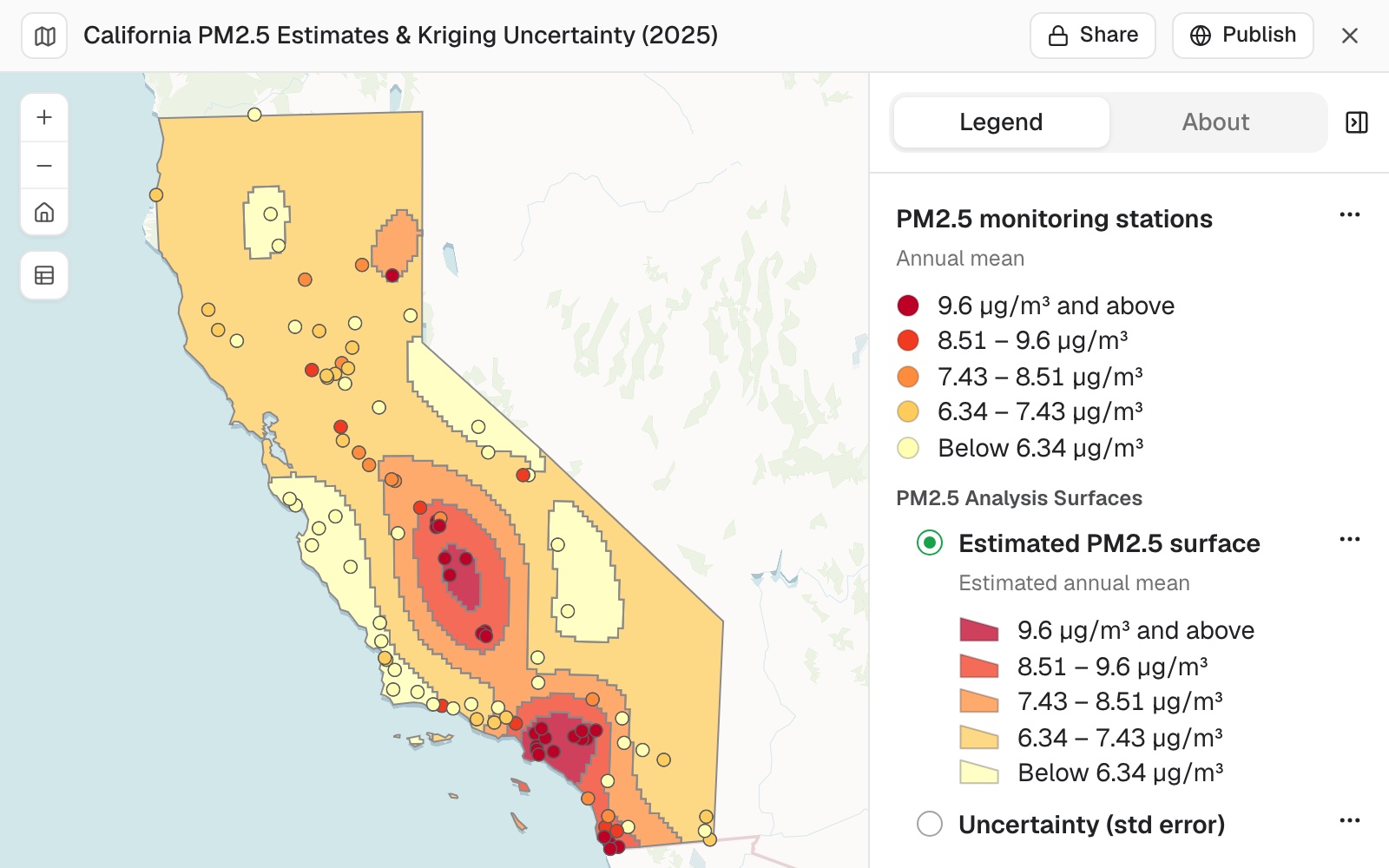 Example: the estimated PM2.5 surface from all 101 monitors in five bands, with each monitor coloured by its own reading on the same scale. The error surface sits beside it in the legend, one shown at a time.
You test how much the picture depends on the samples
Ask what happens if you leave readings out, especially any you are unsure of:
Leave out the 14 sites marked incomplete and run it again. How much does the picture change?
Mapstack reran it on the 87 complete sites, replaced the surfaces on the map and gave a table of what changed: the range of estimates widened to 4.52–11.95 µg/m³ and the error dropped near monitors.
You look at the shape, not only the numbers
A summary table can hide a change in shape. In the example the second surface was a flat background with rings around each monitor. Ask why:
The second surface is a flat background with rings around each monitor, quite unlike the first run. Why, and which run should I trust?
Mapstack explained that without the 14 sites the fitted variogram reached only a short distance (about 45 km, against about 200 km with all 101), so away from a monitor the estimate fell back to the statewide average (the "bullseye" pattern). It recommended the 101-site surface for showing spatial pattern, with a note that 14 sites missed the completeness rule, and the 87-site set where the readings must meet the regulatory completeness standard. Which to use is your call; it depends on what the map is for.
You ask questions of the surface
Which counties have most of their area above 9 µg/m³ in the estimate?
Mapstack fetched the county boundaries, overlaid them on the estimate and measured the area above the threshold in each. In the example the first answer came from the 87-site surface, the one made last: none, with Los Angeles and Kings counties highest at 22%. On the 101-site surface the answer is two: all of Orange County and 66% of Kings County, with Los Angeles County next at 46%. When you have more than one surface in a session, say which one a question is about.
Common questions
How many sample points do I need?
At least 10 with a value in the column you name. With fewer, Mapstack says so; check the column, or add samples.
Why doesn't the surface reach my highest readings?
Kriging smooths: between samples, the estimate is a weighted average of the readings around it. Read the readings themselves for the peaks, and the surface for the pattern between them.
Why does the surface look like rings around each point?
The fitted variogram sees little likeness between readings beyond a short distance, so away from a sample the estimate falls back to the average. Ask how the variogram was fitted, and compare with a run on more points.
How do I check the surface?
Ask how it was set up: the variogram, the grid and the range of the estimates. Look at the error layer, which is high far from the samples. Then leave out readings you doubt and run it again, to see how much the picture depends on them.